Beginners Guide to Pathfinding Algorithms
By ai-depot | December 19, 2002
Optimal Search Methods
Blind searches will find ANY path. Heuristic searches will (usually) find ANY path, but will do so faster (usually) than blind search.
Sometimes it’s OK to find just ANY path to the goal as long as you get there. But sometimes you want to find the BEST path to the goal. The fastest, cheapest, or easiest route to take is oftentimes more important than finding SOME path. Thats where optimal search comes in. The methods that follow are intended to find the optimal path.
The first method is an exhaustive search. This method is guaranteed to find the best path, but is often quite inefficient. The method is simple and, at first glance, logical: explore every possible path and return the shortest one. One way to do this is to do BFS or DFS, but dont stop when the goal is reached. Continue until EVERY node has been visited. During this, though, keep track of the distances traveled on each path and return the shortest one.
This is practical for only small problems as this can get quite computationally expensive very fast.
However, this is not much different than blind searches, so why not add a bit of heuristic tuning to improve efficiency as we have done before? We can expand shortest paths first (as in Best-First Search) and we can stop exploring certain paths if it hasnt reached the goal yet but is still longer than an existing complete path. The end result of this is called Branch and Bound search.
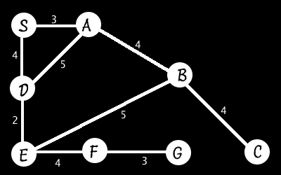
I’ll demonstrate on a new graph:

First, S is added with distance 0. Note that this is the distance TRAVELLED now, rather than the estimated distance to goal.
S is expanded to S->A (with distance travelled = 3) and S->D (distance=4). These are then sorted so the shortest current path is first. This is S->A(3) first.
S->A(3) is expanded to S->A->B(3 + 4 (the distance from A to B) is 7) and S->A->D(8) both are added to the list which is then sorted S->D(4), S->A->B(7), S->A->D(8)
Expanding the shortest one, S->D(4), yields S->D->A(9) and S->D->E(6). The latter of these two happens to have the shortest path now, so we expand that one on the next iteration yielding: S->D->E->B(11) and S->D->E->F(10)
S->A->B is the shortest now, with 7. Expanding this gives us S->A->B->C(11) and S->A->B->E(12).
(for brevity, I’ll list the following steps in this form: [Shortest path] expands to [list of resulting paths])
- S->A->D(8) yields S->A->D->E(10)
- S->D->A(9) yields S->D->A->B(13)
- S->D->E->F(10) yields S->D->E->F->G(13) which means we’ve found the goal with a cost of 13!
Now, as we begin expanding the rest of the paths, we can discard any that give us a cost of greater than 13. S->A->D->E(10) is the current cheapest at this step. We expand it to S->A->D->E->B(15) and S->A->D->E->F(14) Since both are greater than 13, we ignore them.
And so on. It turns out that 13 IS the shortest cost path and our Branch and Bound program found it. I know you’ve been dying for the Branch and Bound psuedocode, so here it is:
 create a list P
 add the start node S, to P giving it one element
 Until first path of P ends with G, or P is empty
        extract the first path from P
        extend first path one step to all neighbors creating X new paths
        reject all paths with loops
        add each remaining new path to of P
        Sort all paths by current distance travelled, shortest first.
 If G found -> success. Else -> failure.
Now we’re going to improve Branch and Bound by adding an underestimate of the remaining distance to the goal. This gives us an underestimate of the total distance of the path:
Total underestimate = current distance travelled + underestimate of distance remaining
We can therefore stop expanding paths if the path’s total underestimate is of greater distance than that of a complete path already found. Underestimates must yield the shortest possible path (shortest distance between two points is a straight line so we use that as our underestimate heuristic).
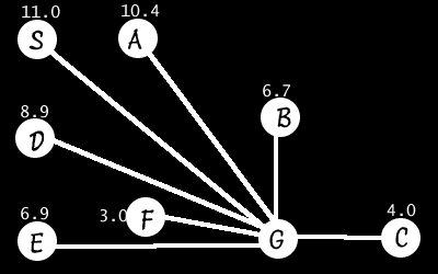
We’ll use the graph above, plus the following straight-line distances:

Now, we keep track of a total underestimate: the total distance travelled, plus the straight-line distance from the last node in the path to the goal.
We expand S(0 distance travelled + 11 underestimate = 11) to S->A(3 + 10.4 = 13.4) and S->D(12.9)
S->D(12.9) has a shorter underestimate than S->A(13.4), so we expand that one. S->D->A(19.4) and S->D->E(12.9) result.
S->D->E(12.9) expands to S->D->E->B(17.7) and S->D->E->F(13)
S->D->E->F(13) Expands to the goal at S->D->E->F->G(13) and we’ve reached our goal with a cost of 13. This is the same thing we got before, but this one took a lot fewer steps and didnt explore nearly as many paths. After we reach the goal with a cost of 13, all other partially explored paths have an estimated cost of greater than 13 so they cant possibly have a lower cost than the path we’ve already found. So, we can safely ignore them.
 create a list P
 add the start node S, to P giving it one element
 Until first path of P ends with G, or P is empty
        extract the first path from P
        extend first path one step to all neighbors creating X new paths
        reject all paths with loops
        add each remaining new path to of P
        Sort all paths by total underestimate, shortest first.
 If G found -> success. Else -> failure.
The total underestimate, again, is: distance of partial path travelled + straight-line distance from last node in path to goal
This seems pretty good and, as it turns out, this is the optimal path for this graph. There is another way to improve efficiency, however, and that is to avoid doing the same work twice. We can do this using Dynamic Programming.
If we implement Branch and Bound with Dynamic Programming, we can see this in action (using the same graph). In this example, we’re looking only at distance travelled again. We’ll return to underestimates shortly.

As usual, we expand S to S->A and S->D. These have partial paths of 3 and 4 respectively.
S->A(3) expands to S->A->B(7) and S->A->D(8) We already had a path go to D, though with the path S->D(4). Since we have a shorter path to D, we can ignore the longer path and discard S->A->D(8).
S->D(4) expands to S->D->A(9) and S->D->E(6) Again, S->D->A(9) is a longer path to A than simply S->A(3) so we can discard it.
S->D->E(6) expands to S->D->E->B(11) and S->D->E->F(10) We discard S->D->E->B(11) because we already have a shorter path to B and continue
S->A->B(7)expands to S->A->B->C(11) and S->A->B->E(12) Since we’ve reached E with half that cost, we discard this longer path.
S->D->E->F(10) expands to S->D->E->F->G(13) and we’ve reached our goa, again with the shortest path.
 create a list P
 add the start node S, to P giving it one element
 Until first path of P ends with G, or P is empty
        extract the first path from P
        extend first path one step to all neighbors creating X new paths
        reject all paths with loops
                for all paths that end at the same node, keep only the shortest one.
        add each remaining new path to of P
        Sort all paths by total distance travelled, shortest first.
 If G found -> success. Else -> failure.
Now, the dynamic programming saved us some steps from the first examples, but not as many as the second (with underestimates). Since we have two different methods of saving us steps, wouldnt it be great if we could combine them some how?
You (and the rest of the AI community) are in luck! Combining Branch and Bound with dynamic programming and underestimates yields the favorite A* pathfinding algorithm.
 create a list P
 add the start node S, to P giving it one element
 Until first path of P ends with G, or P is empty
        extract the first path from P
        extend first path one step to all neighbors creating X new paths
        reject all paths with loops
                for all paths that end at the same node, keep only the shortest one.
        add each remaining new path to of P
        Sort all paths by total underestimate, shortest first.
 If G found -> success. Else -> failure.
If you’ve forgotten, the total underestimate is: distance of partial path travelled + straight-line distance from last node in path to goal
As you can see, A* is the culmination of several time and step-saving techniques which have arisen over the years.
Written by Senior Diablo.
Tags: none
Category: tutorial |

