Path-Planning from Start to Finish
By ai-depot | June 30, 2002
Single Source Algorithms
As the concept of single source algorithms was only glossed over in the previous page, it needs to be explored in more detail before moving on to a specific implementation.
Essentially, the solution to a single source shortest path problem on a graph G is a list of n-1 paths and their respective lengths. The most convenient, and a succinct representation of this solution is a minimum spanning tree. This is a tree data-structure containing all the nodes of the graphs, and only the edges needed for the shortest paths.
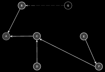
Shortest paths can be built by reverse traversal of the tree, starting from the end point and moving towards the root. The length of that path can either be cached, or computed during the traversal.
Relaxation
This is not a Zen meditation technique, but a procedure that is applied to the graph to form a minimum spanning tree. Essentially, each edge is scanned iteratively. If its end node is further than its start node plus the length of the path, then we update the information stored at that node. This involves resetting the parent node, and changing the distance.
In C++ pseudo-code, this looks a bit like this:
// root node assumed valid
Node* root;// reset all the nodes’ information
for (Node* n = nodes.begin(); n != nodes.end(); n++)
{
n->distance = MAX_FLOAT;
n->parent = root;
}// set properties of root node
root->distance = 0.0;
root->parent = NULL;// start relaxation algorithm
while (!graph.isSpanningTree())
{
// scan all the edges in the graph
for (Edge* e = edges.begin(); e != edges.end(); e++)
{
const float d = e->start->distance + e->length;
// check if distance using this path is better
if (e->end->distance > d)
{
// if so, update the end node
e->end->distance = d;
e->end->parent = e->start;
}
}
}
Depending on how your graph is laid out in memory, this algorithm can be more or less efficient. At the worst, however, it takes a whopping O(2^m) computation time. That’s to be expected from na�ve implementations, and that leaves a lot of room for better algorithms…
Prototypes
Dijkstra was one of the first to really make his mark in the field, by formalising the problem and proposing his initial solution in 1959. This set the premise for a great number of successors, all of which improve the original performance. The concepts behind all the algorithms have, however, been captured into a single “prototype” algorithm — based on Gallo and Pallottino’s work (1986).
Such a prototype would have this appearance:
/**
* Initialise all nodes and the root as in relaxation algorithm above.
*/// create the working list of nodes
vector temporary;
temporary.push_back( root );// start shortest-path algorithm
while (!temporary.empty())
{
// fetch the next node to be scanned
Node* node = Select( &temporary );
// scan all the edges of this node
for (Edge* e = node->edges.begin(); e != node->edges.end(); e++)
{
const float d = e->start->distance + e->length;
// check if distance using this path is better
if (e->end->distance > d)
{
// if so, update the end node
e->end->distance = d;
e->end->parent = e->start;
// this node needs to be processed by the algorithm too
Insert( &temporary, e->end );
}
}
}
The key points lie obviously in the unexplained Select and Insert procedures. In what order do we select the nodes? And how do we store the nodes for efficient insertion and removal? That’s what it’s all about, and looking into Dijkstra’s approach will enlighten us with the first technique used.
Dijkstra’s Algorithm
Dijkstra’s algorithm uses a greedy approach to the node selection; the closest node to the root is selected next. This is known as a best first approach. If this is respected throughout, and if the path-lengths are always positive, then once a node is removed it does not need to be processed again — ever. This property was discovered by Dijkstra, and implemented as such (note that the Insert is not needed):
/**
* Same initialisation as prototype algorithm above.
*/while (!temporary.empty())
{
// fetch the next node to be scanned
Node* node = DeleteMin( &temporary );
// scan all the edges of this node
for (Edge* e = node->edges.begin(); e != node->edges.end(); e++)
{
const float d = e->start->distance + e->length;
// check if distance using this path is better
if (e->end->distance > d)
{
// if so, update the end node
e->end->distance = d;
e->end->parent = e->start;
}
}
}
Improvements
In the initial implementation, the DeleteMin procedure used a linear scan of a list of nodes. This was of computational complexity O(n), providing a simple implementation. No doubt Dijkstra has identified this issue, and considered the upgrade to a more suited data-structure trivial ;)
In following work, Johnson and Dial respectively used d-Heaps and buckets to reduce this complexity notably. Any reasonable data-structure will allow an efficient enough implementation on modern computers, so try to keep things simple!
Tags: none
Category: tutorial |
